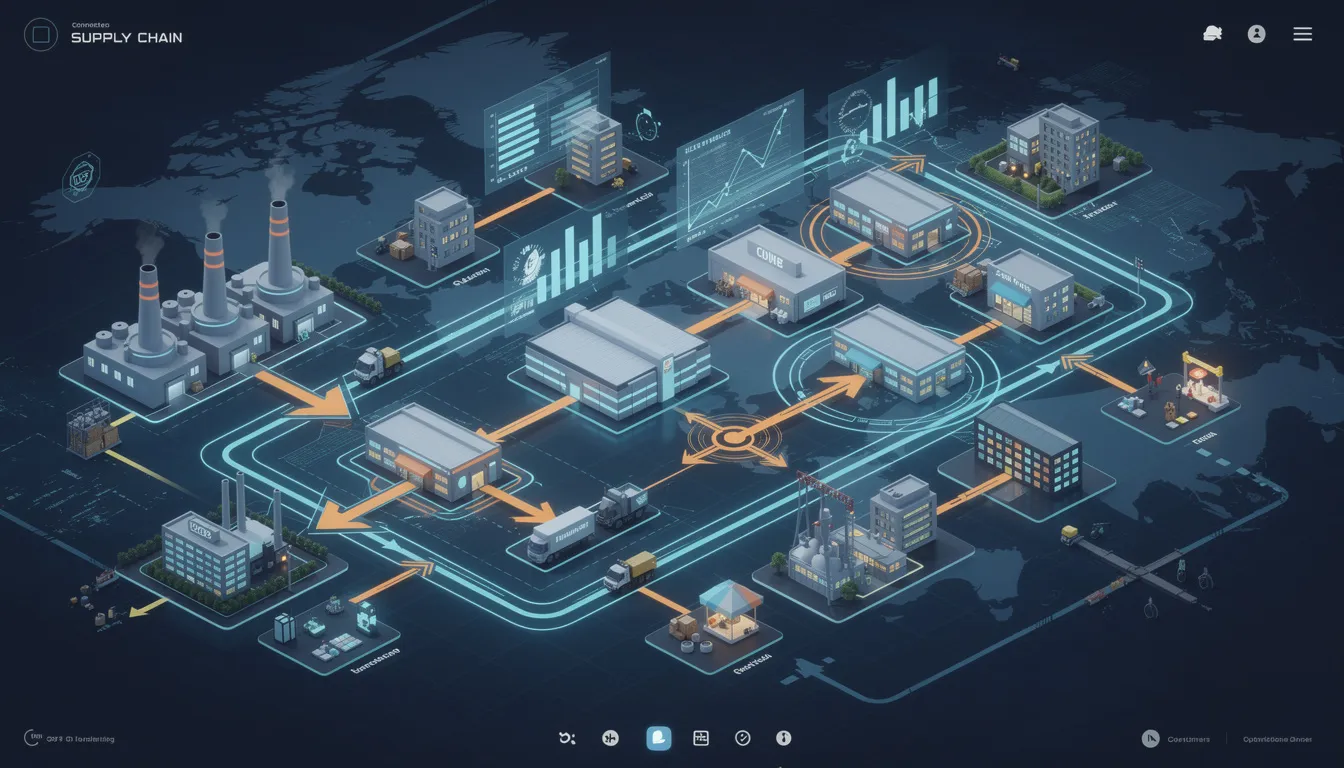
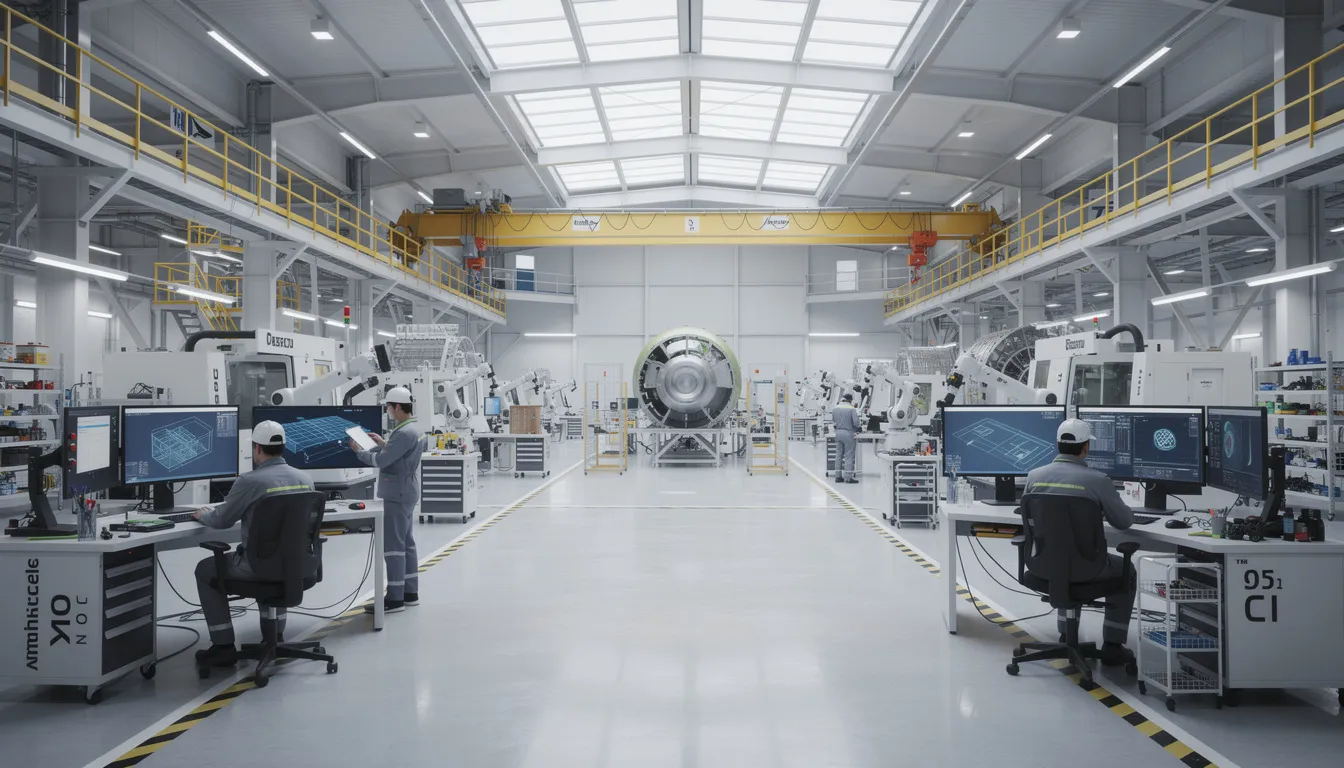
Manufacturing enterprises operating across multiple sites, suppliers, and jurisdictions face a persistent challenge: how to describe what happens between business planning and the physical processes on the factory floor. The answer, for many global organizations, lies in IEC 62264.
This international standard series provides a common framework for enterprise control system integration, giving manufacturers a shared vocabulary for how enterprise systems and control systems exchange information. For aerospace organizations coordinating production, maintenance, and quality operations across complex supply chains, IEC 62264 offers a neutral reference that supports consistent communication regardless of geography or technology platform.
This blog post examines the scope and purpose of IEC 62264, its relationship to ISA 95, and its role in global manufacturing operations.
What Is IEC 62264 in Manufacturing Operations?
IEC 62264 is the internationally adopted version of the ISA-95 enterprise and control system integration standard, focused specifically on manufacturing operations management at Level 3 in the hierarchical model. Published by the International Electrotechnical Commission, IEC 62264 provides a common reference model for how business planning and logistics systems (Level 4) interact with manufacturing operations and control functions (Levels 3 and 2).
The standard exists to serve as a globally recognized counterpart to the ISA-95 series originally developed by the International Society of Automation. While ISA-95 carries ANSI/ISA designation, IEC 62264 enables organizations worldwide to reference the same technical content through their national or regional standards frameworks.
IEC 62264 is widely applied in discrete, batch, and continuous manufacturing sectors. It holds particular relevance for aerospace and MRO operations that rely on interconnected systems including enterprise resource planning, manufacturing execution systems, product lifecycle management, and quality management systems. These environments require precise coordination of production orders, maintenance records, traceability data, and compliance documentation across multiple facilities and suppliers.
Connect981 is a platform built for aerospace manufacturing and MRO teams that aligns to IEC 62264 and ISA-95 concepts. Its approach to organizing digital work instructions, traceability, and supplier workflows reflects the levels, information flows, and terminology established by these standards.
Scope and Purpose of IEC 62264
IEC 62264 defines models, terminology, and interfaces that describe how enterprise systems and manufacturing operations exchange information. It does not prescribe specific technologies or software products. Instead, it provides a conceptual framework that allows different stakeholders, vendors, and sites to interpret and design systems consistently.
The core scope centers on control system integration, specifically the interactions between:
Level
Domain
Examples
Level 4
Business planning and logistics
ERP, supply chain planning, order management
Level 3
Manufacturing operations management
MES, MOM, production scheduling, quality management
Level 2
Supervisory control
SCADA, DCS, supervisory systems
Level 1
Sensing and manipulating
Sensors, actuators, devices
Level 0
Physical processes
Actual production equipment and physical assets
The purpose of IEC 62264 is to standardize how manufacturing activities, information objects, and information flows are described. This standardization allows organizations to map their existing systems into a common reference architecture without requiring a complete technology overhaul.
For aerospace and MRO organizations, this scope supports consistent handling of:
- Production orders and work schedules
- Maintenance orders and equipment states
- Quality data and inspection records
- Materials, lot tracking, and serialization
- Resource allocation across plants and suppliers
The standard’s purpose is informational and modeling-oriented. It defines activity models and object models. It does not mandate how those models should be implemented in any specific technology or business processes.
Relationship Between IEC 62264 and ISA-95
IEC 62264 and ISA 95 cover the same conceptual territory. They were developed in close coordination, with IEC 62264 effectively mirroring the content of ISA-95 for international use.
ISA-95 was first developed and published by ISA in the mid-1990s and early 2000s. The standard addressed a critical functional gap: the interface between enterprise functions operating at Level 4 and process control functions operating at Level 2. When this content achieved sufficient technical maturity, it was adopted and published by the IEC as the IEC 62264 series to provide a global electrotechnical standard.
The part structure aligns closely between the two series:
ISA-95 Part
IEC 62264 Part
Focus Area
ISA-95 Part 1
IEC 62264-1
Models and terminology, Level 3-4 interface
ISA-95 Part 2
IEC 62264-2
Object model attributes
ISA-95 Part 3
IEC 62264-3
Activity models of MOM
ISA-95 Part 4
IEC 62264-4
Object models and attributes
ISA-95 Part 5
IEC 62264-5
Business-to-manufacturing transactions
Conceptually, both series share the same hierarchical model defined for organizing manufacturing levels, the same object models for entities like materials and equipment, and the same activity models for production, maintenance, quality, and inventory operations. Document layouts and editorial details may differ between ISA and IEC publications, but the technical substance remains equivalent.
Connect981’s information model and workflows are designed to be understandable in both ISA-95 and IEC 62264 terms. This helps aerospace teams collaborate across global partners who may refer to either naming convention.
Why IEC Versions Exist Alongside ISA Standards
ISA is a professional society. IEC is a formal international standards body recognized by many national standards organizations and regulators. This distinction explains why both designations exist for the same technical content.
IEC 62264 exists to provide the ISA-95 concepts in a format that can be adopted as national or regional electrotechnical standards. In Europe, for example, CENELEC can adopt IEC standards directly. Other national committees worldwide follow similar processes. When organizations reference IEC 62264, they reference a standard with formal international standing.
Several practical factors drive this dual publication approach:
- Procurement and contracts: Many countries and procurement frameworks reference IEC standards explicitly. Having IEC 62264 makes it easier for multinational manufacturers to align on a single international reference.
- Regulatory alignment: Different jurisdictions have different standards bodies. IEC publication provides equal weight across multiple regulatory environments.
- Community coordination: The coexistence of ISA-95 and IEC 62264 allows both automation professionals and national standards bodies to work from a harmonized conceptual base while following their own publication processes.
This dual publication is especially important in global industries such as aerospace. OEMs, Tier-1 suppliers, and MRO providers must coordinate standards language across multiple jurisdictions. A supplier in Germany can reference IEC 62264 knowing that a customer in the United States recognizes the same technical content under the ISA-95 designation.
How IEC 62264 Mirrors ISA-95 Conceptually
The technical content of IEC 62264 is designed to be conceptually equivalent to ISA-95. Models, definitions, and terminology align across both series by design.
Both standards use a hierarchical view of manufacturing based on the Purdue Reference Model. This layers defined structure organizes technology and business processes from physical production (Level 0) up through business planning (Level 4). The hierarchy provides a common reference for discussing where different systems and functions operate.
In both ISA-95 and IEC 62264, Level 3 (Manufacturing Operations Management) breaks into four key activity areas:
Activity Area
Scope
Production operations
All the activities related to converting materials into products
Maintenance operations
Activities taking place to maintain equipment availability
Quality operations
Activities related to measuring and verifying product and process quality
Inventory operations
Activities for managing materials and storage
Both series define similar object models for entities such as:
- Material (material lots, sublots, serial numbers)
- Equipment (work centers, production units, storage zones)
- Personnel (qualifications, assignments)
- Process segments (routing steps, operations)
These object models enable consistent descriptions of what is being planned, executed, and recorded across manufacturing operations domain applications.
Connect981 uses these same conceptual objects and levels. Work orders, routing, resources, and quality records map cleanly to IEC 62264 and ISA-95 aligned architectures. This alignment makes it easier to integrate enterprise system data with shopfloor execution.
IEC 62264 Part Structure for Manufacturing Operations
IEC 62264 is organized into multiple parts, each addressing a specific aspect of enterprise and control integration. Understanding this structure helps organizations locate the relevant models and terminology for their needs.
IEC 62264-1: This part establishes the foundational framework, including the five-level hierarchy, the manufacturing operations management domain definition (Level 3), and the interfaces between Level 3 and Level 4. The latest edition includes extended functional and equipment hierarchies, a physical asset equipment model, and generic models of manufacturing operations management categories. The interface content describes what information flows between manufacturing operations and other enterprise functions.
IEC 62264-2: Focuses on object model attributes for information exchanges between enterprise and control domain systems.
IEC 62264-3:2016: The second edition defines activity models of manufacturing operations management. It covers production operations management, maintenance operations management, quality operations management, and inventory operations management. The 2016 update consolidated information and aligned terminology with other parts.
IEC 62264-4: Covers object models and attributes used in manufacturing operations, specifying the precise data structures for data exchange between functions.
IEC 62264-5: Addresses business-to-manufacturing transactions, defining how to enable enterprise system communication with manufacturing operations management systems.
The updates across editions have focused on aligning terminology across parts and maintaining consistency with ISA-95 equivalents. Aerospace organizations often use Level-3 activity and object models as a reference for aligning ERP order management, MES systems, and shopfloor execution tools like Connect981.
IEC 62264-3:2016 and Manufacturing Operations Management (MOM)
IEC 62264-3:2016 is the second edition that defines activity models of Manufacturing Operations Management (MOM). It clarifies the role of Level 3 as the operational layer between business planning (Level 4) and control (Level 2).
The activity models in IEC 62264-3:2016 provide a structured way to describe what Level 3 actually does. The models cover:
- Production operations management: Detailed production scheduling, production dispatching, production execution management, and production data collection
- Maintenance operations management: Maintenance scheduling, dispatching, execution, and tracking
- Quality operations management: Quality test management, inspection coordination, and quality data collection
- Inventory operations management: Material movement, storage management, and inventory tracking
These models operate independently of any specific software or hardware. They can describe both traditional MES implementations and newer digital operations platforms. The purpose is to enable information collection and coordination across manufacturing activities regardless of the underlying technology.
This edition updated terminology and cross-references to align with IEC 62264-1 and IEC 62264-4. Activity descriptions and object models use consistent naming across the entire standard series.
Connect981 aligns its features with these MOM activity areas. Digital work instructions, traceability, quality checks, and supplier workflows map to the production, quality, and maintenance operations described in IEC 62264-3:2016. This mapping helps aerospace teams describe their processes using standards-aligned language.
Terminology and Consistency Between IEC 62264 and ISA-95
One of the key aims of both IEC 62264 and ISA-95 is to provide a stable, shared vocabulary for enterprise-control system integration. This interface terminology allows different organizations to describe the same operations the same way.
The two series coordinate on terminology for key concepts:
Term
Definition
Manufacturing Operations Management
Level 3 functions that manage manufacturing operations
Process segment
A logical grouping of manufacturing operations
Material lot
A specific quantity of material with common properties
Equipment
Physical assets used in manufacturing
Work center
A grouping of equipment for production purposes
Production schedule
A plan for production activities over time
Revisions such as those in IEC 62264-3:2016 have explicitly updated terms to align with naming conventions in other parts (for example, IEC 62264-4) and with their ISA-95 counterparts. This deliberate alignment ensures models and terminology remain consistent across the entire standard family.
This terminology consistency allows documentation, system specifications, and cross-site process descriptions to remain coherent whether a stakeholder references the ISA or IEC designation. When different parties in a supply chain use the same terms for the same concepts, integration becomes more straightforward.
Connect981 uses this standards-aligned vocabulary in its data model and user interfaces where practical. This helps aerospace and MRO organizations describe the same operations the same way across OEMs, suppliers, and regulators.
Role of International Standardization in Manufacturing Operations
International standardization through bodies like the IEC enables manufacturers, technology providers, and regulators across different regions to share a common framework for describing manufacturing operations. This role is especially important for industries with global supply chains.
IEC 62264 supports interoperability by giving different systems a shared reference for how information should be structured at the boundaries between business and manufacturing. When an ERP system needs to communicate with an MES, or when an MES needs to exchange data with a QMS, IEC 62264 provides the conceptual framework for describing what information should flow and how it should be structured.
In global aerospace supply chains, this international alignment is crucial for coordinating:
- Production schedules across multiple manufacturing sites
- Quality data shared between OEMs and suppliers
- Maintenance records for aircraft components across MRO providers
- Compliance documentation required by different regulatory authorities
International standards make it easier for software platforms to interoperate with existing systems. Because the information flows can be modeled using widely understood IEC 62264 and ISA-95 concepts, integration projects can proceed from a shared reference point rather than custom definitions.
IEC 62264’s role is to provide a neutral, well-defined language for manufacturing operations. This supports long-term consistency even as specific technologies, architectures, and tools evolve. The standard organizes technology choices without mandating them.
IEC 62264, Smart Manufacturing, and Aerospace Digital Operations
IEC 62264’s models connect directly to current themes such as smart manufacturing, Industry 4.0, and connected aerospace operations. The standard’s technology-agnostic architecture remains valid as organizations adopt new capabilities.
Similar to ISA-95, IEC 62264 offers an architecture that accommodates:
- IoT devices and sensor networks at Levels 0-2
- Cloud analytics and reporting systems
- AI-driven insights and predictive analytics
- Digital thread initiatives connecting design through production
- Automation across manufacturing and quality processes
Aerospace and MRO organizations can use IEC 62264 concepts to describe how information should move between:
- Planning systems: Build plans, maintenance programs, production schedules
- Operations systems: Work execution, inspections, resource allocation
- Supporting systems: Configuration management, certification records, audit trails
The hierarchical model and activity models provide a stable reference even as the underlying technology changes. An organization can modernize its industrial control systems, adopt new information technology platforms, or implement advanced automation while maintaining alignment with the same conceptual framework.
Platforms like Connect981 implement digital work instructions, traceability, supplier collaboration, and real-time reporting in ways that fit naturally into the Level 3 Manufacturing Operations Management space described by IEC 62264-3. This alignment provides several advantages:
- Clear boundaries between what enterprise systems manage and what shopfloor systems manage
- Consistent terminology for describing product offerings and system capabilities
- A reference for how information should flow between applications performing business functions and those managing physical production
By aligning digital operations platforms with IEC 62264 and ISA-95 concepts, aerospace manufacturers and MRO providers can modernize their operations while keeping a clear, standards-aligned structure for information and responsibilities. The result is operations that increase uniformity across sites and suppliers without requiring all parties to use identical technology platforms.
IEC 62264 provides the neutral, well-defined language that global aerospace manufacturing operations require. Its conceptual mirroring of ISA-95 ensures that organizations referencing either designation work from the same technical foundation. For aerospace teams coordinating production, maintenance, quality, and supply chain activities related to complex product offerings, this standards alignment supports consistent communication across other domains and systems.
Connect981 is designed with these IEC 62264 and ISA-95 concepts in mind, organizing digital aerospace manufacturing and MRO workflows around the same levels, objects, and activities that the standards describe. To see how this standards-aligned approach works in practice, request a demo and explore how Connect981 fits into your operations architecture.